Kalman Filter
Thank You Michel van Biezen
It’s an iterative mathematical process that uses a set of equations and consecutive data inputs to quickly estimate the actual value of the object being measured, when the measured value contain random error.
Let’s say, we want to measure temperature with a certain thermometer and that thermometer is not very accurate.
In the figure above, y-axis represents temperature while x-axis represents time. The little crosses are consecutive inputs. We can see that the temperature measured has a certain amount of uncertainty and therefore, it will take us a long time to average these values out. Kalman filter can do this lot faster.
It starts out by taking an initial estimate, it almost doesn’t matter what that initial estimate is. In the estimate, we need to predict a certain amount of error but as data points start coming in and we go through the iterative process, the Kalman filter narrows down to somewhere close to the true value very quickly.
Temperature is a single value but if we want to track a satellite, then we would need it’s location and velocity in both x and y directions.
Three main calculations:
Kalman Gain
Current Estimate
New error in estimate
The figure on the left gives an overview of the process for conducting Kalman filtering.
The 3 calculations are to be performed in an iterative manner for the estimate to zoom in the actual value.
To calculate the gain, we need error in estimate which would be either previous or original. We also need error in the input which we are getting continuously.
Gain puts relative importance in the error in the estimate versus the error in the data. If error in estimate is smaller, we put more importance in it and vice versa.
After calculating the gain, it is fed into calculate the current estimate. It also depends on previous or original estimate and the data input. Gain will decide how much weight to put in on the new measured value or on the previous estimate.
Next, we need to calculate the new error in estimate and we need current estimate and gain to calculate it.
Kalman Gain is basically what is used to determine how much of the new measurements to use to update the new estimate.
Kalman Gain is the ratio of the error in the estimate divided by the sum of the error in the estimate plus the error in the measurement. It is always between 0 and 1.
If the Kalman Gain is high, it means that the measurements we are getting are fairly accurate and the estimates are unstable.
If the error in the measurement is less, we want to contribute much of the update to the current or new estimate by the measurement and vice versa.
For each iteration, we calculate the Kalman Gain, new estimate and error in estimate, combined with their formulas are shown in the figure above.
Error in estimate is basically the inverse of Kalman Gain multiplied by the previous error in estimate.
If the Kalman Gain is large that means error in the measurement is small which means that new data put in can now very quickly get us to the true value and therefore we will reduce the error in the estimate and vice versa.
Example
For an experiment, error in measurement remains same if the conditions don’t change. Initial setting for a numerical example is shown in the figure above.
First iteration is shown in the figure above.
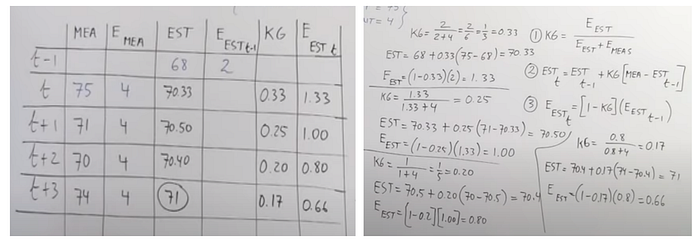
After only 4 iterations, we are able to reach 71 which is very close to 72 being the actual value.
